The standard nudging method has been widely studied in the past decades [69,109,103,102]. Thus, there are several ways to choose the nudging matrix ![]() in the forward part of the algorithm. One can for example consider the optimal nudging matrix
in the forward part of the algorithm. One can for example consider the optimal nudging matrix ![]() , as discussed in [119,112]. In such an approach, a variational data assimilation scheme is used in a parameter estimation mode to determine the optimal nudging coefficients. This choice theoretically provides the best results for the forward part of the BFN scheme, but the computation of the optimal gain matrix is costly.
, as discussed in [119,112]. In such an approach, a variational data assimilation scheme is used in a parameter estimation mode to determine the optimal nudging coefficients. This choice theoretically provides the best results for the forward part of the BFN scheme, but the computation of the optimal gain matrix is costly.
When ![]() , the forward nudging problem (3.2) simply becomes the direct model (3.1). On the other hand, setting
, the forward nudging problem (3.2) simply becomes the direct model (3.1). On the other hand, setting ![]() forces the state variables to be equal to the observations at discrete times, as is done in [105,104]. These two choices have the common drawback of considering only one of the two sources of information (model and data).
forces the state variables to be equal to the observations at discrete times, as is done in [105,104]. These two choices have the common drawback of considering only one of the two sources of information (model and data).
Let us assume that we know the statistics of errors on observations, and denote by ![]() the covariance matrix of observation errors. This matrix is involved in all standard data assimilation, either variational (3D-VAR, 4D-VAR, 4D-PSAS, ...) or sequential (Kalman filters) [52,59,90,65,66]. Usually, it is impossible to know the exact statistics of errors, and thus only an approximation of
the covariance matrix of observation errors. This matrix is involved in all standard data assimilation, either variational (3D-VAR, 4D-VAR, 4D-PSAS, ...) or sequential (Kalman filters) [52,59,90,65,66]. Usually, it is impossible to know the exact statistics of errors, and thus only an approximation of ![]() is available, assumed to be symmetric positive definite.
is available, assumed to be symmetric positive definite.
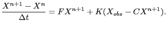
We assume here the direct model to be linear (or linearized). We consider a temporal discretization of the forward nudging problem (3.2), using for example an implicit scheme. If we denote by ![]() the solution at time
the solution at time ![]() and
and ![]() the solution at time
the solution at time ![]() , and
, and
![]() , then equation (3.2) becomes
, then equation (3.2) becomes
We now set the nudging matrix to be
As a consequence, there is no need to consider an additional term ensuring an initial condition close to the background state like in variational algorithms, neither for stabilizing or regularizing the problem, nor from a physical point of view. One can simply initialize the BFN scheme with the background state, without any information on its statistics of errors.
The nudging method naturally provides a correction to the model equations from the observations. The model equations are hence weak constraints in the BFN scheme. In some nonlinear cases, the
![]() term in equation (3.9) can be replaced by
term in equation (3.9) can be replaced by ![]() , where
, where ![]() is the energy of the system at equilibrium.
is the energy of the system at equilibrium.
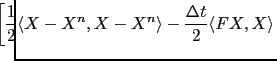
![$\displaystyle \hspace*{-0.5cm} + \left. \frac{\Delta t}{2} \langle R^{-1}(X_{obs}-CX),X_{obs}-CX\rangle \right].$](img264.png)