We consider here a linear situation, although simple, that describes quite well how the BFN algorithm works. We assume that the observation operator ![]() is equal to the identity, and that the model
is equal to the identity, and that the model ![]() is linear. We also assume that
is linear. We also assume that ![]() and
and ![]() commute. Note that this assumption is valid in our experiments as
commute. Note that this assumption is valid in our experiments as ![]() is set proportional to the identity matrix. In this pretty simple situation, we can explicit the BFN trajectories. For the sake of concision and clarity, we assume that
is set proportional to the identity matrix. In this pretty simple situation, we can explicit the BFN trajectories. For the sake of concision and clarity, we assume that ![]() , but the following results remain valid if
, but the following results remain valid if ![]() . We finally assume that the length of the assimilation period is
. We finally assume that the length of the assimilation period is ![]() .
.
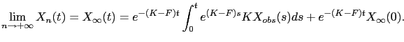
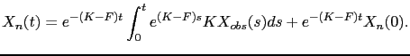
Then, for all ![]() ,
,
 |
|||
| (3.19) |
 |
(3.20) |
The following result proves the existence of a limit trajectory [20]:
Under the same hypothesis, we have a similar result for backward trajectories, i.e. there exists a function
![]() such that
such that
![]() , for all
, for all
![]() . This proves the convergence of the BFN algorithm in such a situation.
. This proves the convergence of the BFN algorithm in such a situation.
Note that the limit function
![]() (resp.
(resp.
![]() ) is totally independent of the initial condition
) is totally independent of the initial condition ![]() of the algorithm.
of the algorithm.
Moreover, if the observations are perfect, i.e. ![]() satisfies the direct model equation (3.1), then for all
satisfies the direct model equation (3.1), then for all
![]() ,
,
| (3.23) |
| (3.24) |
The BFN algorithm also has a similar behaviour on linear parabolic operators in infinite dimension (e.g. the heat operator). A Fourier decomposition of the trajectories allows us to study only first order ordinary differential equations, and gives then the convergence of the algorithm.