Extension to color images

Next: Classification Up: Restoration Previous: Remarks Contents

Extension to color images

In this section, we adapt the topological gradient approach to color images. Color images can be represented or modeled in various ways, for instance the RGB (Red-Green-Blue) space in which images are viewed as functions from $\Omega$ to $\mathbb{R}^3$ instead of $\mathbb{R}$ . A first approach consists of decoupling the three channels, and in solving direct and adjoint problems for each channel. But it is also possible to consider directly the vectorial minimization problem, involving the resolution of vectorial problems. The topological asymptotic expansion is still given by equations (2.25-2.26) and (2.28), where all functions are vectorial, i.e. the topological gradient is the sum on all channels of the corresponding expressions for each channel [25].

Another approach has also been studied in [25], in which we use a different norm for coupling the different channels. In order to identify the local variations of the color image, Di Zenzo defines a multi-spectral tensor associated to the image vector field [55]:

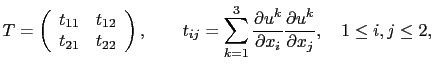$\displaystyle T = \left( \begin{array}{cc} t_{11} & t_{12} \\ t_{21} & t_{22} \... ...rtial u^k}{\partial x_i}\frac{\partial u^k}{\partial x_j}, \quad 1\le i,j\le 2,$

(2.30)

in the case of bidimensional images. This tensor describes the first order differential structure of the image, and the Di Zenzo gradient is given by the square root of the largest eigenvalue of the structure tensor:

$\displaystyle \Vert\nabla u\Vert _{DZ} = \frac{1}{\sqrt{2}} \left[ t_{11}+t_{22}+\sqrt{(t_{11}-t_{22})^2+4t_{12}^2}\right]^{\frac{1}{2}}.$

(2.31)

It is possible to rewrite this gradient in a different way with the following function:

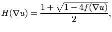$\displaystyle H(\nabla u) = \frac{1+\sqrt{1-4f(\nabla u)}}{2},$

(2.32)

where

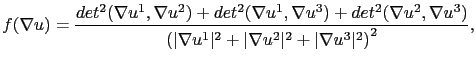$\displaystyle f(\nabla u) = \frac{det^2(\nabla u^1,\nabla u^2)+det^2(\nabla u^1... ...\nabla u^1\vert^2 + \vert\nabla u^2\vert^2 + \vert\nabla u^3\vert^2 \right)^2},$

(2.33)

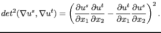$\displaystyle det^2(\nabla u^s,\nabla u^t) = \left( \frac{\partial u^s}{\partia... ...2}-\frac{\partial u^t}{\partial x_1}\frac{\partial u^s}{\partial x_2}\right)^2.$

(2.34)

Then, we can derive the asymptotic expansion of the cost function defined by equation (2.24) in which the norm is the Di Zenzo norm (2.31):

$\displaystyle G(x_0,n) = \sum_{k=1}^3 \left[ -\pi c (\nabla u_0^k(x_0).n)(\nabla v_0^k(x_0).n)-\pi H(\nabla u_0(x_0))\vert\nabla u_0^k(x_0).n\vert^2\right]$

(2.35)

with our standard notations.

In [25], we show that this approach has the same computational cost as the vectorial approach (in which the different channels are decoupled), while it improves the edge detection, and hence it produces a better restored image, more precise on the edges of the image.

Next: Classification Up: Restoration Previous: Remarks Contents

Back to home page