next up previous contents
Next: Power series expansion Up: Segmentation Previous: Segmentation   Contents

From restoration to segmentation

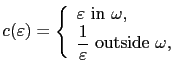
We still consider the restoration algorithm, in which the following conductivity is used for the perturbed problem:

$\displaystyle c(\varepsilon) = \left\{ \begin{array}{l} \varepsilon \textrm{ in...
...isplaystyle\frac{1}{\varepsilon} \textrm{ outside } \omega, \end{array} \right.$ (2.40)

where $ \omega\subset\Omega$ represents the edge set. We first assume that $ \omega$ is thickened (i.e. of codimension 0 in $ \Omega$ ). From equation (2.40), the algorithm now consists of solving the following problem:

$\displaystyle (\mathcal{P}_\varepsilon)\ \ \left\{ \begin{array}{lll} -div(\var...
...mega,\\ \partial_n u_\varepsilon = 0 & on & \partial\Omega, \end{array} \right.$ (2.41)

where $ u_\varepsilon\in H^1(\Omega)$ , i.e. with the implicit boundary condition that $ c(\varepsilon)\partial_n u_\varepsilon$ has the same value on both sides of $ \partial\omega$ .

Then we have the following asymptotic result [18]:

Theorem 2.2   If we denote by $ u_\varepsilon$ the unique solution of problem $ (\mathcal{P}_\varepsilon)$ in $ H^1(\Omega)$ , then

$\displaystyle \lim_{\varepsilon\to 0} (\Vert\nabla u_\varepsilon - \nabla u_0\V...
...^2(\Omega\backslash\omega)} + \Vert u_\varepsilon-u_0\Vert _{L^2(\omega)}) = 0,$ (2.42)

where $ u_0\in H^1(\Omega\backslash\omega)\cap L^2(\Omega)$ is the solution to the following problem

$\displaystyle (\mathcal{P}_0)\ \ \left\{ \begin{array}{lll} u_0 = v & in & \ome...
...\partial\omega,\\ \partial_n u_0 = 0 & on & \partial\Omega. \end{array} \right.$ (2.43)

This result proves that the segmented image $ u_0$ can be approximated by $ u_\varepsilon$ if $ \varepsilon$ is small. We now assume that the edge set $ \omega$ is of codimension $ 1$ in $ \Omega$ . From the point of view of applications, it is completely natural to assume that the edges are flat in the image. In order to have coherent notations, we will further denote by $ \sigma$ the edge set. We assume that $ \sigma$ is known, e.g. provided by the crack detection algorithm previously seen.

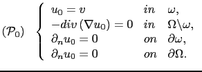
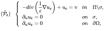
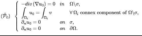
We can rewrite the approximated segmentation problem $ (\mathcal{P}_\varepsilon)$ as follows:

$\displaystyle (\tilde{\mathcal{P}}_\varepsilon)\ \ \left\{ \begin{array}{lll} \...
...igma,\\ \partial_n u_\varepsilon = 0 & on & \partial\Omega, \end{array} \right.$ (2.44)

where $ u_\varepsilon\in H^1(\Omega\backslash\sigma)$ . If $ v\in L^2(\Omega)$ , then problem $ (\tilde{\mathcal{P}}_\varepsilon)$ has a unique solution in $ H^1(\Omega\backslash\sigma)$ . As a corollary of the previous result, we have the following one [18]:

Theorem 2.3   If we denote by $ u_\varepsilon$ the unique solution of problem $ (\tilde{\mathcal{P}}_\varepsilon)$ in $ H^1(\Omega\backslash\sigma)$ , then

$\displaystyle \Vert u_\varepsilon\Vert _{L^2(\Omega)}\le\Vert v\Vert _{L^2(\Ome...
..._{L^2(\Omega\backslash\sigma)}\le\sqrt{\varepsilon}\Vert v\Vert _{L^2(\Omega)},$ (2.45)

and

$\displaystyle \lim_{\varepsilon\to 0} \Vert\nabla u_\varepsilon - \nabla u_0\Vert _{L^2(\Omega\backslash\sigma)} = 0,$ (2.46)

where $ u_0\in H^1(\Omega\backslash\sigma)$ is the unique solution to the following problem:

$\displaystyle (\tilde{\mathcal{P}}_0)\ \ \left\{ \begin{array}{lll} -div\left(\...
... & on & \sigma,\\ \partial_n u_0 = 0 & on & \partial\Omega. \end{array} \right.$ (2.47)

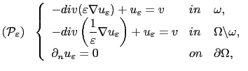
For numerical reasons, it can be very difficult to solve directly problem $ (\tilde{\mathcal{P}}_0)$ , and even problem $ (\tilde{\mathcal{P}}_\varepsilon)$ for too small values of $ \varepsilon>0$ . Indeed the conditioning of the system to be solved goes to infinity when $ \varepsilon\to 0$ . In order to overcome this issue, we will expand the solution $ u_\varepsilon$ of problem $ (\tilde{\mathcal{P}}_\varepsilon)$ into a power series of $ \varepsilon$ .


next up previous contents
Next: Power series expansion Up: Segmentation Previous: Segmentation   Contents
Back to home page