Discrete cosine transform

Next: Preconditioned conjugate gradient Up: Complexity and speeding up Previous: Complexity and speeding up Contents

Discrete cosine transform

In all the algorithms we presented in the previous sections, we only have to solve the following PDE

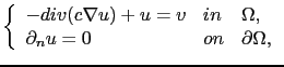$\displaystyle \left\{ \begin{array}{lll} -div(c\nabla u)+u=v & in & \Omega,\\ \partial_n u = 0 & on & \partial\Omega, \end{array} \right.$

(2.54)

for various coefficients

. The first resolutions are done with a constant value of

. It is then possible to largely speed up the computation time by using the discrete cosine transform (DCT) method. Problem (2.54) is then equivalent to

$\displaystyle \sum_{m,n} \left( 1+c(m\pi)^2+c(n\pi)^2\right) u_{m,n}\phi_{m,n} = \sum_{m,n} v_{m,n}\phi_{m,n},$

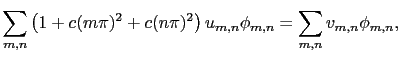(2.55)

where we denote by 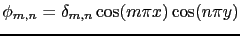$\phi_{m,n}=\delta_{m,n} \cos(m\pi x)\cos(n\pi y)$ a cosine basis of $\mathbb{R}^2$ , and where $(v_{m,n})$ represent the DCT coefficients of the original image

. It is then straightforward to identify $(u_{m,n})$ , the DCT coefficients of

in equation (2.55):

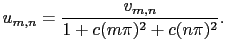$\displaystyle u_{m,n} = \frac{v_{m,n}}{1+c(m\pi)^2+c(n\pi)^2}.$

(2.56)

The complexity of such a resolution is $\mathcal{O}(n.\log(n))$ , where

is the number of pixels of the image. The resolution of all unperturbed problems is then done in the following way:

$\bullet$: Computation of $v_{m,n}$ , the DCT coefficients of the original image .
$\bullet$: Computation of $u_{m,n}$ , the DCT coefficients of from equation (2.56).
$\bullet$: Computation of using an inverse DCT.

Next: Preconditioned conjugate gradient Up: Complexity and speeding up Previous: Complexity and speeding up Contents

Back to home page