


Next: BFN algorithm
Up: ``Back and Forth Nudging''
Previous: Forward nudging
Contents
We now assume that we have a final condition in equation (3.1) instead of an initial condition. This leads to the following backward equation:
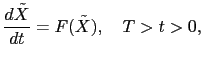 |
(3.3) |
with a final condition
 . The backward nudging algorithm consists of solving backwards in time the state equations of the model, starting from the observation of the system state at the final time [15]. If we apply nudging to this backward model with a feedback term of the opposite sign (in order to have a well posed problem), we obtain
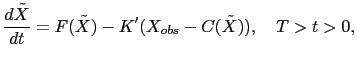 |
(3.4) |
where  is the backward nudging matrix.
The backward integration of this equation provides a state vector at time  , which can be seen as an identified initial condition for our data assimilation period.
Back to home page