The back and forth nudging algorithm, introduced in [20], consists of first solving the forward nudging equation and then the backward nudging equation. The initial condition of the backward integration is the final state obtained after integration of the forward nudging equation. At the end of this process, one obtains an estimate of the initial state of the system. We repeat these forward and backward integrations (with the feedback terms) until convergence of the algorithm:
If ![]() and if the forward and backward trajectories
and if the forward and backward trajectories ![]() and
and
![]() converge towards the same limit trajectory
converge towards the same limit trajectory
![]() , then it is clear by adding the two equations of (3.5) that
, then it is clear by adding the two equations of (3.5) that
![]() also satifies the model equation (3.1), and that
also satifies the model equation (3.1), and that
![]() .
.
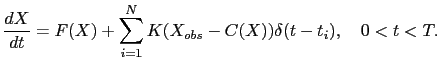
When the observations are discrete in time, i.e. the observation vector ![]() is only available at some times
is only available at some times
![]() , then the nudging term is only added at these time steps:
, then the nudging term is only added at these time steps:
![\begin{displaymath}\begin{array}{l} k\ge 1\quad \left\{ \begin{array}{l} \displa...
...0.2cm] \tilde{X}_k(T) = X_k(T), \end{array} \right. \end{array}\end{displaymath}](img241.png)