


Next: Experimental approach
Up: Numerical experiments
Previous: Numerical experiments
Contents
All numerical experiments have been performed with an easy-to-implement nudging matrix:
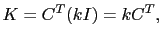 |
(3.11) |
where  is a positive scalar gain, and
  is the identity matrix of the observation space. This choice is motivated by the following remarks. First, the covariance matrix of observation errors is usually not well known (but if it is available, then one should consider equation (3.8) for the definition of
  ). Secondly, this choice does not require a costly numerical integration of a parameter estimation problem for the determination of the optimal coefficients. Choosing
  , where
  is a square matrix in the observation space, has another interesting property: if the observations are not located at a model grid point, or are a function of the model state vector, i.e. if the observation operator
  involves interpolation/extrapolation or some change of variables, then the nudging matrix
will contain the adjoint operations, i.e. some interpolation/extrapolation back to the model grid points, or the inverse change of variable.
involves interpolation/extrapolation or some change of variables, then the nudging matrix
will contain the adjoint operations, i.e. some interpolation/extrapolation back to the model grid points, or the inverse change of variable.
As in the forward part of the algorithm, for simplicity reasons we make the following choice for the backward nudging matrix  :
:
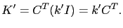 |
(3.12) |
The only parameters of the BFN algorithm are then the coefficients
and  . In the forward mode,
  is usually chosen such that the nudging term remains small in comparison with the other terms in the model equation. The coefficient
is usually chosen to be the smallest coefficient that makes the numerical backward integration stable.
is usually chosen such that the nudging term remains small in comparison with the other terms in the model equation. The coefficient
is usually chosen to be the smallest coefficient that makes the numerical backward integration stable.
Next: Experimental approach
Up: Numerical experiments
Previous: Numerical experiments
Contents
Back to home page