We have finally considered a layered quasi-geostrophic ocean model [70,110,39]. This model arises from the primitive equations (conservation laws of mass, momentum, temperature and salinity), assuming first that the rotational effect (Coriolis force) is much stronger than the inertial effects. The Rossby number, ratio between the characteristic time of the Earth's rotation and the inertial time, must then be small compared to ![]() . Second, the thermodynamic effects are completely neglected in this model. Quasigeostrophy assumes that the horizontal dimension of the ocean is small compared to the size of the Earth, with a ratio of the order of the Rossby number. We finally assume that the depth of the basin is small compared to its width. In the case of the Atlantic Ocean, not all these assumptions are valid, notably the horizontal extension of the ocean. But it has been shown that the quasi-geostrophic approximation is fairly robust in practice, and that this approximate model reproduces quite well the ocean circulations at mid-latitudes, such as the jet stream (e.g. Gulf Stream in the case of the North Atlantic Ocean) and ocean boundary currents.
. Second, the thermodynamic effects are completely neglected in this model. Quasigeostrophy assumes that the horizontal dimension of the ocean is small compared to the size of the Earth, with a ratio of the order of the Rossby number. We finally assume that the depth of the basin is small compared to its width. In the case of the Atlantic Ocean, not all these assumptions are valid, notably the horizontal extension of the ocean. But it has been shown that the quasi-geostrophic approximation is fairly robust in practice, and that this approximate model reproduces quite well the ocean circulations at mid-latitudes, such as the jet stream (e.g. Gulf Stream in the case of the North Atlantic Ocean) and ocean boundary currents.
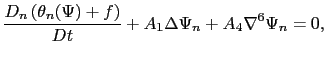
The model system is then composed of ![]() coupled equations resulting from the conservation law of the potential vorticity. The equations can be written as:
coupled equations resulting from the conservation law of the potential vorticity. The equations can be written as:
![]() is the circulation basin,
is the circulation basin, ![]() is the stream function at layer
is the stream function at layer ![]() ,
, ![]() is the sum of the dynamical and thermal vorticities at layer
is the sum of the dynamical and thermal vorticities at layer ![]() ,
, ![]() is the Coriolis force, and the dissipative terms correspond to the lateral friction and the bottom friction dissipation. Finally,
is the Coriolis force, and the dissipative terms correspond to the lateral friction and the bottom friction dissipation. Finally, ![]() is the forcing term of the model, the wind stress applied to the ocean surface. We refer to [70,110,39] for more details about this model and its equations.
is the forcing term of the model, the wind stress applied to the ocean surface. We refer to [70,110,39] for more details about this model and its equations.
We refer to [21] for the reports of numerical simulations on this model: convergence, comparison with the 4D-VAR algorithm, sensitivity studies, ...
![$\displaystyle \frac{D_1\left( \theta_1(\Psi)+f \right)}{Dt}+A_4 \nabla^6\Psi_1=F_1 \quad \textrm{in } \Omega \times ]0,T[,$](img298.png)
![$\displaystyle \frac{D_k\left( \theta_k(\Psi)+f \right)}{Dt}+A_4 \nabla^6\Psi_k=0 \quad \textrm{in } \Omega \times ]0,T[,$](img300.png)