


Next: Invariant correction terms
Up: Nudging and observers
Previous: Nudging and observers
Contents
We consider here a shallow water model, similar to the model introduced in section 3.3.3. However, the equations are rewritten in order to clearly see the symmetries. We refer to [72] for more details about these equations. In the following,  is the fluid height, and
  is the bi-dimensional velocity field. The equations write:
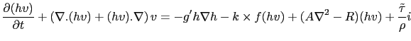 |
(3.48) |
for the vectorial velocity, and
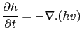 |
(3.49) |
for the scalar height. In these equations,  represents the reduced gravity,
  is the fluid density,
  is the Coriolis parameter,
  is the longitudinal unit vector (pointing towards East) and
  is the upward unit vector. Finally,
  ,
,  and
and
 represent friction, lateral viscosity, and the forcing term (zonal wind stress) respectively.
We assume that the physical system is observed by several satellites that provide measurements of the sea surface height (SSH)
only.
An observer
 for the system (3.48-3.49) writes:
 |
(3.50) |
and
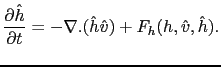 |
(3.51) |
The only difference between the observer and model equations comes from the innovation terms
 and
and
 . The correction terms must vanish when the estimated height
  is equal to the observed height
. The goal is to define functions
is equal to the observed height
. The goal is to define functions  and
and  such that the observer tends to the true solution. Moreover, these feedback terms also have to preserve the symmetries of the model.
Next: Invariant correction terms
Up: Nudging and observers
Previous: Nudging and observers
Contents
Back to home page