In order to avoid the amplification of the measurement noise by a differentiation process, only the integral correction terms are kept: one sets
![]() ,
, ![]() and
and
![]() .
.
For the sake of clarity, we now simplify the model equations, by assuming that there is no Coriolis force, no friction, no dissipation, and no wind stress. An observer for this simplified system satisfies then:
Note that in the degenerate case where
![]() and
and
![]() ,
, ![]() and
and ![]() being positive scalars, we find the standard nudging terms, or Luenberger observer.
being positive scalars, we find the standard nudging terms, or Luenberger observer.
As it seems difficult to first study the convergence on the nonlinear system, we now linearize the equations around an equilibrium position ![]() and
and ![]() . We only consider small velocities
. We only consider small velocities
![]() and heights
and heights
![]() , where
, where ![]() and
and ![]() represent the equilibrium height and speed respectively. We denote by
represent the equilibrium height and speed respectively. We denote by ![]() (resp.
(resp. ![]() ) the estimation errors, differences between the observer and true solution, for the height (resp. velocity). These errors are solution of the following linear equations:
) the estimation errors, differences between the observer and true solution, for the height (resp. velocity). These errors are solution of the following linear equations:
A reasonable choice for the kernels ![]() and
and ![]() is the following:
is the following:
| (3.64) | |||
| (3.65) |
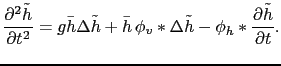
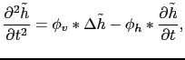
Eliminating the velocity ![]() in equations (3.60-3.61) leads to a modified damped wave equation with external viscous damping:
in equations (3.60-3.61) leads to a modified damped wave equation with external viscous damping:
 |
(3.67) |
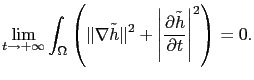
Then, we have the following result [22]:
 |
(3.69) |
A dimensional analysis also provides the following gain tuning (see equations (3.62) and (3.69)):
| (3.70) |