The minimization of the cost function ![]() is performed in nested subspaces:
is performed in nested subspaces:
| (4.11) |
The difference with hierarchical techniques issued from the optical flow family (see e.g. [84,92]) is that we do not linearize the cost function. This should help to find large displacements, where the domain of linearity of the luminance function is not valid.
The space
![]() is typically of small dimension, hence the minimization of
is typically of small dimension, hence the minimization of ![]() on
on
![]() is fast and robust when a zero vector field is used as initial guess. The optimal vector field obtained at a given scale in the space
is fast and robust when a zero vector field is used as initial guess. The optimal vector field obtained at a given scale in the space
![]() is used as initial guess to find the minimum at the finer scale in the space
is used as initial guess to find the minimum at the finer scale in the space
![]() . This process is iteratively repeated, until an optimal solution is identified on the finest grid.
. This process is iteratively repeated, until an optimal solution is identified on the finest grid.
All the optimizations of the nonlinear cost function are performed by a Gauss-Newton method. When an initial guess ![]() is given (a constant null field, in our experiments), the
is given (a constant null field, in our experiments), the ![]() -th iteration read
-th iteration read
| (4.12) |
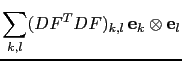
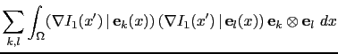
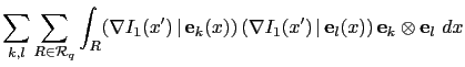
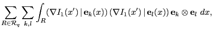
Another innovation of the present work is the efficient computation of the product ![]() of the Jacobian of the first term of the cost function (4.2) by its transpose. This efficient computation comes from the observation that this matrix is sparse and can be assembled like a finite-element matrix using one loop over the data.
of the Jacobian of the first term of the cost function (4.2) by its transpose. This efficient computation comes from the observation that this matrix is sparse and can be assembled like a finite-element matrix using one loop over the data.
Let
![]() be a vector field. Let
be a vector field. Let
![]() be the canonical orthonormal basis of
be the canonical orthonormal basis of
![]() , containing vector fields that are equal to 0
at every but one control point, where the vector field is directed along the horizontal or vertical axis. The
, containing vector fields that are equal to 0
at every but one control point, where the vector field is directed along the horizontal or vertical axis. The
![]() coefficient of the matrix
coefficient of the matrix ![]() is
is
| (4.14) |
| (4.15) |
Finally, equation (4.13) is solved using a conjugate gradient method wihtout preconditioning.