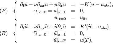
We now consider the viscous Burgers' equation, a standard nonlinear transport equation. We also consider only one iteration of the BFN algorithm:
In the particular case where
![]() , the backward problem is ill-posed in the sense of Hadamard (the solution does not depend continuously on the data), but it has a unique solution if the final condition
, the backward problem is ill-posed in the sense of Hadamard (the solution does not depend continuously on the data), but it has a unique solution if the final condition
![]() is set to a final solution of the direct equation. Moreover, in this particular case, the backward solution is exactly equal to the forward one:
is set to a final solution of the direct equation. Moreover, in this particular case, the backward solution is exactly equal to the forward one:
![]() for all
for all ![]() . The main result is the following [29]:
. The main result is the following [29]:
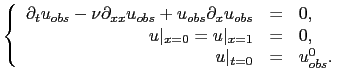
The BFN algorithm is then ill-posed (except if
![]() ) when applied to a viscous Burgers' equation, as there does not exist a solution to the backward problem. However, from the numerical point of view, the BFN algorithm has been successfully applied to this model [21]. This phenomenon is probably due to the fact that we numerically solve a discrete problem and not the exact continuous one.
) when applied to a viscous Burgers' equation, as there does not exist a solution to the backward problem. However, from the numerical point of view, the BFN algorithm has been successfully applied to this model [21]. This phenomenon is probably due to the fact that we numerically solve a discrete problem and not the exact continuous one.